Input files
Configuration parameters
To configure the PlatoSim, a large set of configuration parameters is required. The input file format used for PlatoSim3 is YAML. All configuration parameters and files are read from the default YAML file called inputfile.yaml located in the inputfiles/ directory. The different blocks in the configuration files reflect their function in the simulation. We use only a very limited set of the YAML functionality, enough to allow us to provide input files for different parts of the simulator.
Overview of Configuration Parameters
- General
- Observation
- Sky
- Platform
- Telescope
- Camera
- PSF
- FEE
- CCD
- Subfield
- Photometry
- Random seeds
- Control HDF5 content
- Control TCP connection
- Additionally, there are two blocks that hold predefined settings:
In the following sections we describe these parameters for the simulations in detail. For more details on the reference frames we are using (for the spacecraft, telescope, focal plane, and CCD), radial dependency of the PSF, and rotation angles for platform jitter and camera drift, please, consult the PlatoSim paper and the technical note PLATO-KUL-PL-TN-0001.
General
The general configuration parameters are listed in the General block of the configuration file. The structure of this block is the following:
General:

    ProjectLocation:             ENV['PLATO_PROJECT_HOME']
ProjectLocation: Allowed values Name of exported environment variable
Full path of the directory in which you have checked out the PlatoSim3 project, or an environment variable, e.g. PLATO_PROJECT_HOME, containing the full path to that directory. In the latter case, you must make sure you have exported this variable before using PlatoSim (see prerequisites).
Observing Parameters
The ObservingParameters block of the configuration file contains the configuration parameters that are specific to the simulated observation and are not specific for the hardware components of the satellite. The structure of this block is the following:
ObservingParameters:

  MissionDuration:                 6.5
  NumExposures:                    10
  BeginExposureNr:                 0
  CycleTime:                       25
  Fluxm0:                          1.00179e8
  StarCatalogFile:                 inputfiles/starcatalog.txt
MissionDuration Allowed values \(> 0\) yr
Total duration of the mission, from Beginning Of Life (BOL) to End Of Life (EOL). This will be used to model the parameter degradation over time due to ageing.
NumExposures: Allowed values \(> 0\)
Number of exposures to generate in the simulation.
BeginExposureNr: Allowed values \(> 0\)
Sequential number of the first exposure. Useful for Slurm parallelisation. In that case, long simulations (i.e. with a large number of exposures) will be chopped up into smaller simulations, covering a small number of exposures (see the Fig. 1).
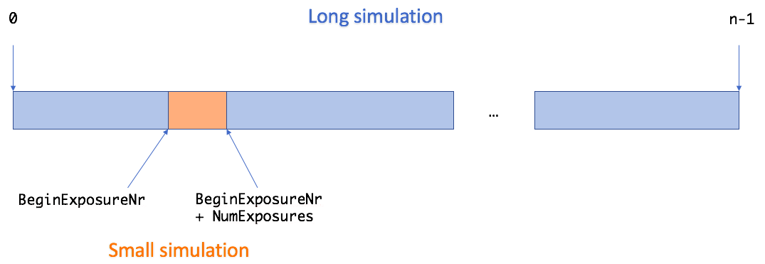
Fig. 1: Long simulations can be chopped up into smaller simulations for parallelisation.
CycleTime: Allowed values \(> 0\) s
Image cycle time. This is the sum of the integration time of one exposure and the subsequent readout:
\(t_{\text{cycle}} = t_{\text{exp}} + t_{\text{readout}}\)
For the normal cameras, the latter is the total readout time; for the fast cameras, it is the time for the frame transfer (i.e. to transfer the content of the upper CCD half to the lower CCD half).
Fluxm0: Allowed values \(> 0 \ \gamma \, \text{s}^{-1} \, \text{cm}^{-2}\)
Flux of a star of zero magnitude (\(m_{\lambda} = 0\)) in the passband of the magnitudes that are listed in the star catalogue below.
For an exposure of \(t_{\rm exp}\) seconds, the measured flux \(F_{\gamma}\) of a star, expressed in photons \(\gamma\), is computed from its catalogue magnitude \(m_{\lambda}\), the effective light-collecting area \(A\) (in \(\text{cm}^2\)) of the telescope, the transmission efficiency \(T_{\lambda}\) of the optical system, the quantum efficiency \(Q_{\lambda}\) of the detector, and the flux per second \(F_0\) of a star with zero magnitude (\(m_{\lambda} = 0\)) from the equation:
\(F_{\lambda} = t_{\rm exp} \ F_0\ T_{\lambda}\ Q_{\lambda} \ A \ 10^{-0.4 \, m_{\lambda}}\)
where the \(\lambda\) refers to the wavelength range in which the simulation is performed.
StarCatalogFile: Allowed values Path to Star Catalog File
Path to the star catalogue file containing three columns, separated by a space, holding the following information:
- Right ascension of the stars [deg]
- Declination of the stars [deg]
- Stellar magnitude (in passband corresponding to
Fluxm0)
A fourth column is optional and should contain positive integers, serving as star identifier. If absent, the line number will act as star identifier (counting starts at 1). Note that by default PlatoSim uses the Long Observational Phase (LOP) South field from the PLATO Input Cata (PIC1.1).
Sky
The Sky block of the configuration file contains all the information that is specific to the sky, i.e. sky background and cosmics. The structure of this block is the following:
SkyBackground:
SkyBackground/UseConstantSkyBackground: Allowed values
yesandnoIf
yesa constant sky background over the entire subfield will be computed. Ifnoa gradient sky background will be computed ifBackgroundValueis set to negative.SkyBackground/BackgroundValue: Allowed values \(\in \mathbb{Z} \, \gamma \, \text{s}^{-1} \, \text{pixel}^{-1}\)
In case a positive value is given (\(>0\)), the sky background, is simply set to the given value over the entire subfield.
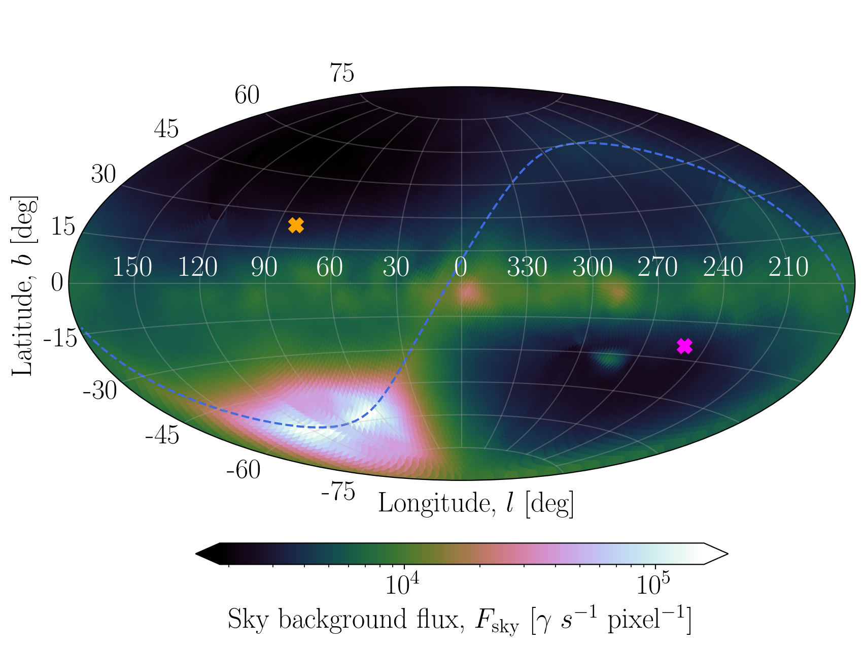
Fig. 2: Aitoff projection of the sky background map in Galactic coordimates.
In case a negative value is given (\(<0\)), the sky background is automatically computed from tabulations of a zodiacal and galactic sky map. Fig. 2 shows the interpolated sky background map used where the blue dashed line is the ecliptica and the orange and magenta crosses are current LOP North and South pointings. Note that the sky background value has not been multiplied with the tranmission efficiency yet.
IncludeVariableSources: Allowed values yes and no
Indicates whether or not stellar variability must be included.
VariableSourceList: Allowed values Path to Variable Source List
In case you want to include stellar variability for the sources in the star catalogue, you must provide an ascii file with two columns, separated by a space:
- Star identifier (the same as in the star catalogue)
- Path to the Variable Source File indicating how the magnitude of this particular source varies over time.
The latter files also consist of two columns separated by a space:
- Time [sec]
- Delta magnitude (with zero mean)
IncludeCosmicsInSubField: Allowed values yes and no
Indicates whether or not cosmics must be added to the pixel map.
IncludeCosmicsInBiasMap: Allowed values yes and no
Indicates whether or not cosmics must be added to the bias register map.
IncludeCosmicsInSmearingMap: Allowed values yes and no
Indicates whether or not cosmics must be added to the smearing map.
Cosmics:
The configuration parameters in the Cosmics section are the parameters characterising the cosmic hits. The excess electrons of the cosmic hits are distributed over a trail, characterised by a decay function of the form:
\(f(t) = \exp{\left(\frac{-t^2}{2 \, \sigma^2}\right)}\)
The following parameters are only applicable if cosmics are included in at least one of the above image maps.
Cosmics/CosmicHitRate: Allowed values \(\geq 0 \, \text{events} \, \text{cm}^{2} \, \text{s}^{-1}\)
Mean cosmic hit rate. The actual cosmic hit rate for any exposure is sampled randomly from a Poisson distribution with the mean cosmic hit rate as mean. The number of cosmic hits in the simulated subfield is calculated by multiplying the actual cosmic hit rate with the size of the subfield and the cycle time.
Cosmics/TrailLength: Allowed values \(> \{0, 0\} \ \text{cm}\)
Interval for the allowed length of the cosmic trails.
Cosmics/Intensity: Allowed values \(> \{0, 0, 0\} \ \text{e}^-\)
Interval for the allowed number of electrons comprised in a cosmic hit (that are to be spread over the trail).
Platform
The Platform block of the configuration file contains all the information that is specific to the platform of the satellite. The structure of this block is the following:
Orientation:
The orientation of the spacecraft can be configured either through the the sky (coordinate) angles (\(\alpha\), \(\delta\), \(\kappa\)) or using a so-called Quaternion.
Angles/RApointing: Allowed values \(\alpha \in [0, 360]\) deg
Right ascension of the platform pointing.
Angles/DecPointing: Allowed values \(\delta \in [-90, 90]\) deg
Declination of the platform pointing.
Angles/SolarPanelOrientation: Allowed values \(\kappa \in [0, 360]\) deg
Orientation angle of the solar panel. This is the roll angle of the platform, which enables orienting the solar panels towards the Sun each quarter, i.e. at the beginning of each quarter the roll angle must be increased by 90 degrees (being either 0, 90, 180, and 270). Note that to properly account for the re-orientation of the solar panels, simulations must be chopped up in chunks of maximum three months (one mission quarter).
Quaternion/Components: Allowed values \(\in [-1, 1]\) for all four component.
A unit quaternion to transform from the equatorial to the platfrom reference frame.
UseJitter: Allowed values yes and no
Indicates whether pointing variations should be taken into account.
PlatoSim can also account for pointing variations of the spacecraft, so-called jitter. A time series of pointing displacement, expressed in Euler angles (yaw, pitch, roll), either has to be provided as a jitter file or will be generated based on the given jitter parameters (see further). To ensure a realistic modelling of the jitter, the time step of the jitter time series must be smaller than the exposure time.
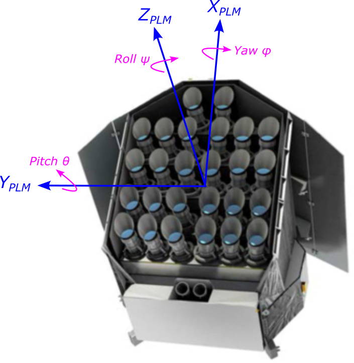
Fig. 3: Platform configuration for AOCS Jitter.
The configuration of the jitter axes is depicted below. The Euler angles that characterise the jitter are defined w.r.t. to the spacecraft coordinate system (see Fig. 3). The origin of this coordinate system is the geometric centre of the interface between the bottom of the optical bench and the service module. The positive roll axis \(Z_{\rm PLM}\) points towards the operator-given mean payload line-of-sight, given by the equatorial coordinates (RApointing, DecPointing, solarPanelOrientation).
The angles are defined such that they increase with a clockwise rotation, when looking along the positive axes. First a roll rotation is done around the \(Z_{\rm PLM}\) axis, then a pitch rotation is done around the rotated \(Y_{\rm PLM}\) axis, and finally a yaw rotation is done around the twice-rotated \(X_{\rm SC}\) axis.
JitterSource: Allowed values FromRedNoise, FromFile, and FromNetwork
Indicates from where to read the jitter:
FromRedNoise: Jitter positions must be generator from the jitter parameters;FromFile: Jitter time series must be read from a jitter file;FromNetwork: Jitter positions must be read from a network (see ControlTcpConnection).
JitterYawRms: Allowed values \(\ge 0\) arcsec
Standard deviation of the normal distribution (with zero mean) describing the yaw value from one jitter position to the next one. This entry is only applicable if JitterSource = FromRedNoise.
JitterPitchRms: Allowed values \(\ge 0\) arcsec
Standard deviation of the normal distribution (with zero mean) describing the pitch value from one jitter position to the next one. This entry is only applicable if JitterSource = FromRedNoise.
JitterRollRms: Allowed values \(\ge 0\)
Standard deviation of the normal distribution (with zero mean) describing the roll value from one jitter position to the next one. This entry is only applicable if JitterSource = FromRedNoise.
JitterTimeScale: Allowed values \(> 0\) s
Timescale of the jitter (i.e. time between two subsequent jitter positions). This entry is only applicable if JitterSource = FromRedNoise.
JitterFileName: Allowed values Path to Jitter File
If JitterSource = FromFile, a jitter time series must be provided in a file ascii format. This file should contain four columns, separated by a space, holding the following information:
- Time [s]
- Yaw [arcsec]
- Pitch [arcsec]
- Roll [arcsec]
Warning
To ensure a realistic modelling of the jitter, the time step in the jitter time series must be smaller than the exposure time.
Telescope
The Telescope block of the configuration file contains all the information that is specific to the telescope. The structure of this block is the following:
GroupID: Allowed values 1, 2, 3, 4, Fast, and Custom
The telescope group identifier can be used to select a camera group. As shown in Fig. 4, there are four groups that have a tilt angle of \(9.2^{\circ}\) - from the optical axis of the satellite, and one group for the fast camera’s which is aligned with the platform \(Z_{\rm PLM}\) axis (black dot of Fig. 4). When you specify GroupID = Custom, the tilt angle and azimuth angle below the GroupID in the inputfile are used, otherwise the angles are taken from predefined parameters in the CameraGroups block of the configuration file.
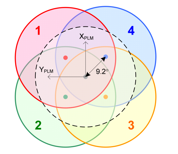
Fig. 4: FOV for the different camera groups.
TiltAngle: Allowed values \(\in [0, 90]\) deg
Tilt angle of the telescope. This angle, together with the azimuth angle, characterises the orientation of the telescope pointing (i.e. telescope optical axis) w.r.t. the platform pointing. This parameter is only used if GroupID = Custom.
The tilt angle is the offset between the camera optical axis and the platform pointing, i.e. the angle between the camera line-of-sight (positive \(Z_{\rm CAM}\) axis and the positive \(Z_{\rm PLM}\) axis (see Fig. 4).
AzimuthAngle: Allowed values \(\in [0, 360]\) deg
Azimuth angle of the telescope, expressed in degrees. This angle, together with the tilt angle, characterises the orientation of the telescope pointing (i.e. telescope optical axis) w.r.t. the platform pointing. This parameter is only used if GroupID = Custom.
The azimuth angle is the position angle of the rotation of the telescope around the positive \(z_{\rm PLM}\) axis (see Figs. 4 and 5).
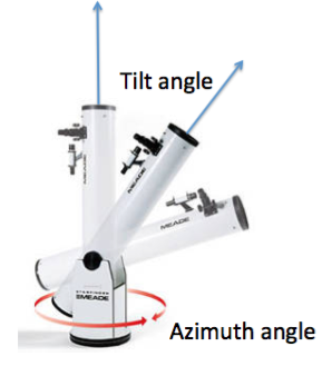
Fig. 5: Tilt and azimuth of camera.
LightCollectingArea: Allowed values \(> 0 \ \text{cm}^2\)
Light-collecting area of one telescope.
TransmissionEfficiency:
The transmission efficiency of the optical system, considering the passband and the spectral energy distribution of the stars, given the Fluxm0 parameter and the magnitudes in the star catalogue degrades linearly over the mission lifetime. The following two parameters are used to model the (linear) degradation in transmission efficiency over the mission lifetime:
TransmissionEfficiency/BOL: Allowed values \(\in [0, 1]\)
Tranmission efficiency of the optical system, considering the passband and spectral energy distribution of the stars, given the
Fluxm0parameter and the magnitudes in the star catalogue, at the beginning of the mission (BOL).TransmissionEfficiency/EOL: Allowed values \(\in [0, 1]\)
Tranmission efficiency of the optical system, considering the passband and spectral energy distribution of the stars, given the
Fluxm0parameter and the magnitudes in the star catalogue, at the end of the mission (EOL).
UseDrift: Allowed values yes and no
Indicates whether the thermo-elastic drift of the camera (w.r.t. the platform) should be taken into account. Similar to the UseJitter parameter for the platform jitter.
PlatoSim can also account for the thermo-elastic drift, of the camera (w.r.t. the platform). A time series of displacements, expressed in Euler angles (yaw, pitch, roll), either has to be provided as a drift file or will be generated based on the given drift parameters shown below.
The Euler angles (yaw, pitch, roll) are defined as the rotation angles around the \(Z_{\rm PLM}\), \(Y'_{\rm PLM}\), and \(Z_{\rm CAM} = Z_{\rm FP}\) axes, such that the anges increase with a clockwise rotation when looking along the positive axes (see Fig. 6).
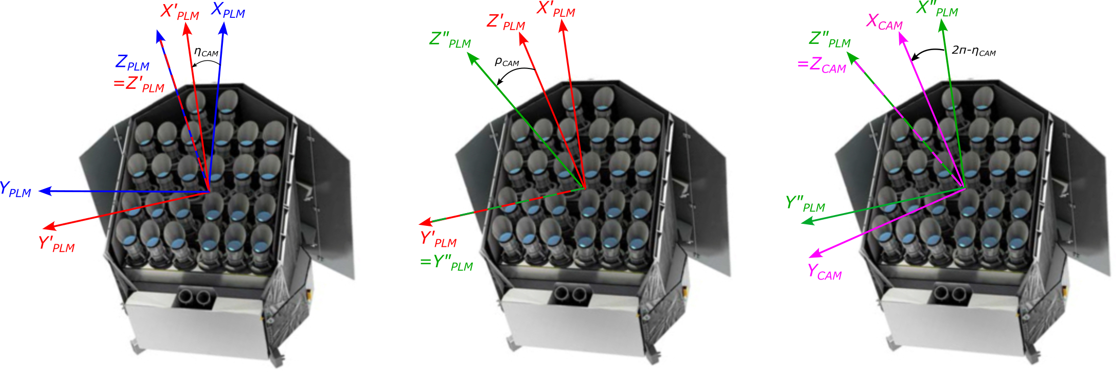
Fig. 6: Reference transformation from the platform to the camera reference system.
The camera reference frame can be obtained from the payload module reference frame by first rotating the \((X_{\rm PLM} \,,Y_{\rm PLM})\) plane around the pointing axis \(Z_{\rm PLM}\) over an angle \(\eta_{\rm CAM}\) (left panel), then rotating the resulting \(Z'_{\rm PLM}\) axis over a tilt angle \(\rho_{\rm CAM}\) around the \(Y'_{\rm PLM}\) axis (middle panel), and finally rotating over an angle \((2π − \eta_{\rm CAM} = -\eta_{\rm CAM})\) around the \(Z''_{\rm PLM}\) (right panel).
DriftSource: Allowed values FromRedNoise and FromFile
Indicates from where to read the drift:
FromRedNoise: the drift positions must be generator from the drift parametersFromFile: the drift time series must be read from a drift file
DriftYawRms: Allowed values \(\ge 0\) arcsec
Standard deviation of the normal distribution (with zero mean) describing the yaw value from one drift position to the next one. This parameter is only used if DriftSource = FromRedNoise.
DriftPitchRms: Allowed values \(\ge 0\) arcsec
Standard deviation of the normal distribution (with zero mean) describing the pitch value from one drift position to the next one. This parameter is only used if DriftSource = FromRedNoise.
DriftRollRms: Allowed values \(\ge 0\) arcsec
Standard deviation of the normal distribution (with zero mean) describing the roll value from one drift position to the next one. This parameter is only used if DriftSource = FromRedNoise.
DriftTimeScale: Allowed values \(> 0\) s
Timescale of the drift (i.e. time between two subsequent drift positions). This parameter is only used if DriftSource = FromRedNoise.
DriftFileName: Allowed values Path to Drift File
If DriftSource = FromFile, camera drift file must be provided in ascii format. This file should contain four columns, separated by a space, holding the following information:
- Time [s]
- Yaw [arcsec]
- Pitch [arcsec]
- Roll [arcsec]
Camera
The Camera block of the configuration file contains all the information that is specific to the camera. The structure of this block is the following:
PlateScale: Allowed values \(> 0 \ \text{arcsec} \, \text{micron}^{-1}\)
Nominal plate scale. This value affects the visible FOV of the CCD.
FocalPlaneOrientation:
The orientation of the focal plane can either be kept constant over the simulations or vary, according to the values in a file provided by the user. For an angle of \(0^{\circ}\), the \(Y_{\rm CCD}\) axis of the CCD (with an orientation angle of \(0^{\circ}\)) points towards the North. A positive angle corresponds to a counter-clockwise rotation. Have a look at Fig. 7 for more details.
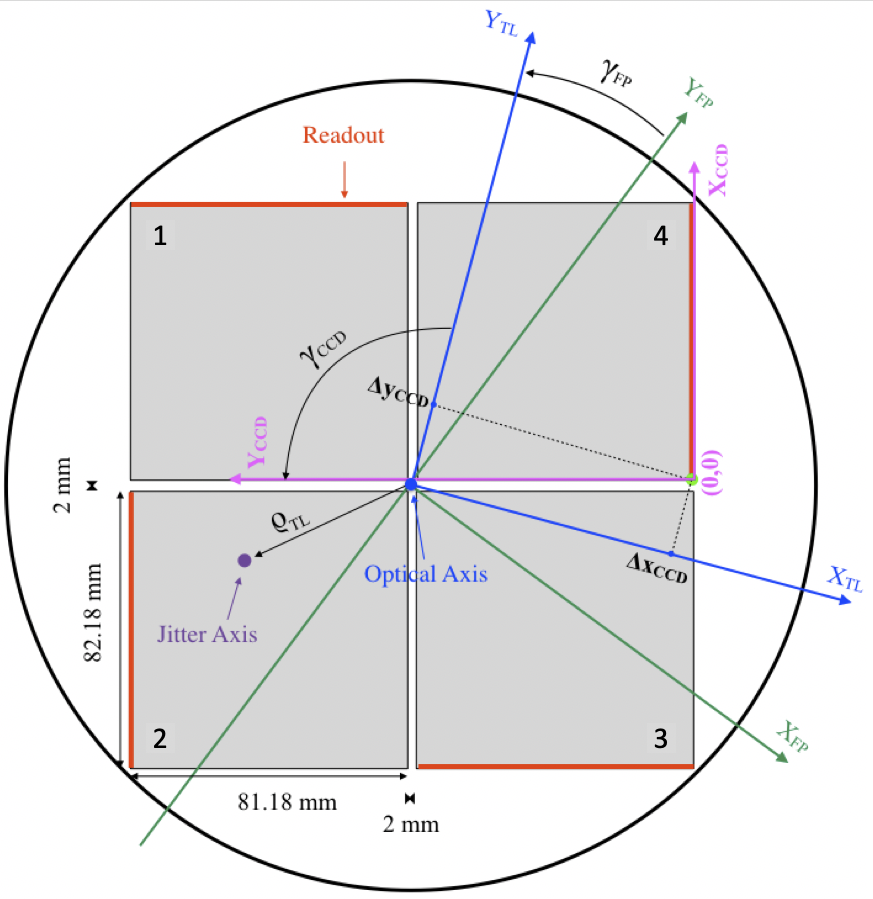
Fig. 7: A schematic overview of the focal plane with 4 CCDs.
The optical axis \(Z_{\rm FP}\) is the blue dot in the middle of the 4 CCDs and points in the positive direction towards the reader. The jitter roll axis \(Z_{\rm CAM}\) is the purple dot, and also points in the positive direction towards the reader. The focal plane is rotated by the angle \(\gamma_{\rm FP}\) w.r.t. to the North direction. The origin of the CCD in the focal plane is defined by its offset \((\Delta X_{\rm CCD}, \Delta Y_{\rm CCD})\) in mm from the centre of the focal plane. It is then rotated by the angle \(\gamma_{\rm CCD}\) round its origin.
FocalPlaneOrientation/Source: Allowed values
ConstantValueandFromFileIndicates whether the value of the focal-plane orientation angle must be constant or is allowed to vary over time, according to the values read from a file.
FocalPlaneOrientation/ConstantValue: Allowed values \(\in [0, 360]\) deg
Orientation angle of the focal plane. This entry is only applicable if
FocalPlaneOrientation/Source = ConstantValue.FocalPlaneOrientation/FromFile: Allowed values Path to Focal Plane Orientation File
If
FocalPlaneOrientation/Source = FromFile, a focal-plane orientation time series must be provided in an acsii file. This file should contain two columns, separated by a space, holding the following information:
- Time [s]
- Focal-plane orientation [deg]
FocalLength:
The focal length can either be kept constant over the simulations or vary, according to the values in a file provided by the user.
FocalLength/Source: Allowed values
ConstantValueandFromFileIndicates whether the value of the focal length must be constant or is allowed to vary over time, according to the values read from a file.
FocalLength/ConstantValue: Allowed values \(> 0\) m
Focal length as recovered from the Zemax model. This entry is only applicable if
FocalLength/Source = ConstantValue.FocalLength/FromFile: Allowed values Path to Focal Length File
If
FocalLength/Source = FromFile, a focal-length time series must be provided in a acsii file. This file should contain two columns, separated by a space, holding the following information:
- Time [s]
- Focal length [m]
ThroughputBandwidth: Allowed values \(> 0\) nm
FWHM of the throughput passband
ThroughputLambdaC: Allowed values \(> 0\) nm
Central wavelength of the throughput passband.
IncludeAberrationCorrection: Allowed values yes and no
Indicates whether or not to apply the aberration correction to all star positions in the star catalogue.
AberrationCorrection:
The calculation of the aberration correction is based on a elliptic earth orbit around the sun and does likewise take the Lissajous orbit of the satellite around L2 into account. We do calculate the kinematic aberration both in an absolute sense and differentially. The latter will be the observant for PLATO data products due to a absolute correction by the fine guidance sensor. The following parameters are only applicable if IncludeAbberationCorrection = yes:
IncludeAberrationCorrection/Type: Allowed values
differentialandabsoluteIndicates whether to apply either differential or absolute aberration correction.
IncludeAberrationCorrection/OrbitFile: Allowed values Path to Orbit File
The orbit file needs to be provided in ascii format and consist of four columns, each seperated by a space:
- Time [s]
- Coordinates of the spacecraft \((x, y, z)\)
- Velocity of the spacecraft \((v_x, v_y, v_z)\) [m/s]
- Speed of the spacecraft [m/s].
IncludeAberrationCorrection/StartTime: Allowed values \(> 0\)
The time at in the orbit file that coresponds with exposure number 0.
IncludeFieldDistortion: Allowed values yes and no
Indicates whether or not the field distortion must be taken into account.
FieldDistortion:
The field distortion is represented by Distortion model from Wang et al. (2007) with coefficients: \((k_1, \, k_2, \, k_3, \, q_1, \, q_2, \, p_1, \, p_2)\). Note that the default distortion coeffcients are only applicable for the Wang model of the N-CAMs used for when PSF/Model = AnalyticNonGaussian (see PSF block).
FieldDistortion/Source: Allowed values
ConstantValueandFromFileIndicates that the field distortion is calculated from a
ConstantVlaue(constant in time) orFromFile(time dependent). The latter needs to be a time series of the field distortion coefficients and their inverse in two files in ascii format.FieldDistortion/ConstantCoefficients: Allowed values \(\in \{\mathbb{R}, \mathbb{R}, \mathbb{R}, \mathbb{R}, \mathbb{R}, \mathbb{R}\}\)
Coefficients for the Wang model that converts the normalised undistorted pixel coordinates (i.e. pixel coordinates divided by the focal length in pixels) to the distortion, expressed in normalised pixel coordinates. This entry is only applicable if
FieldDistortion/Source = ConstantValue.FieldDistortion/ConstantInverseCoefficients: Allowed values \(\in \{\mathbb{R}, \mathbb{R}, \mathbb{R}, \mathbb{R}, \mathbb{R}, \mathbb{R}\}\)
Inverse coefficients for the Wang model that converts the normalised distorted pixel coordinates (i.e. pixel coordinates divided by the focal length in pixels) to the (negative) distortion, expressed in normalised pixel coordinates. This entry is only applicable if
FieldDistortion/Source = ConstantValue.FieldDistortion/CoefficientsFromFile: Allowed values Path to Field Distortion file
If
FieldDistortion/Source = FromFile, a time series of the change in field distortion must be provided in a acsii file. This file should contain two columns, separated by a space, holding the following information:
- Time [s]
- Field distortion coefficients (all separated by spaces)
FieldDistortion/InverseCoefficientsFromFile: Allowed values Path to Inverse Disotion File
If
FieldDistortion/Source = FromFile, a time series of the change in field distortion must be provided in a acsii file. This file should contain two columns, separated by a space, holding the following information:
- Time [s]
- Field distortion inverse coefficients (all separated by spaces)
Ghosts:
Sources in the FOV can produces two types of ghosts:
- a point-like ghost;
- an extended ghost.
The Telescope Optical Unit (TOU) representative of each cameras is shown in Fig. 8.
Fig. 8: A schematic overview the Telescope Optical Unit (TOU). Credit: ESA.
Note that the flux loss of the sources (due to reflection off the CCD surface) is included in the quantum efficiency.
Ghosts/PointLike:
A star at focal-plane coordinates \((x, y)\) will produce a point-like ghost at focal-plane coordinates \((-x, -y)\) (i.e. at the opposite side of the optical axis on another CCD), as long as it is within the distance cut-off from the optical axis. This point-like ghost is caused by reflections on the CCD surface and both window surfaces (see Fig. 8).
Ghosts/PointLike/FluxRatio: Allowed values \(> [0, 1]\)
Irradiance ratio of the point-like ghost w.r.t. the source producing it, measured on-axis. The flux ratio off-axis decreases linearly from the optical axis to the distance cut-off (where it drops to zero), due to vignetting by the pupil around L3. This entry is only applicable if
IncludePointLikeGhost = yes.Ghosts/PointLike/DistanceCutOff: Allowed values \(> 0\) deg
Distance from the optical axis beyond which sources no longer produce point-like ghosts. At this distance, the flux ratio has dropped to zero. This entry is only applicable if
IncludePointLikeGhost = yes.Ghosts/Extended:
A star at focal-plane coordinates \((x, y)\) will produce an extended ghost further away from the optical axis. This ghost image is caused by reflections on the CCD surface and the back surface of L6.
Ghosts/Extended/FluxRatio: Allowed values \(> [0, 1]\)
Irradiance ratio of the extended ghost w.r.t. the source producing it. This entry is only applicable if
IncludeExtendedLikeGhost = yes.Ghosts/Extended/RadiusCoefficients: Allowed values \(> \{0, 0, 0\}\)
Coefficients of the 2nd order polynomial (in distance from the optical axis), describing the radius of the (circular) extended source. This entry is only applicable if
IncludeExtendedLikeGhost = yes.Ghosts/Extended/DistanceRatio: Allowed values \(> 0\) deg
A star at focal-plane coordinates \((x, y)\) will produce a ghost at focal-plane coordinates (
distanceRatio\(\cdot x\),distanceRatio\(\cdot y\)). This entry is only applicable ifIncludeExtendedLikeGhost = yes.
PSF
The PSF block of the configuration file contains all the information that is specific to the PSF. The structure of this block is the following:
Model: Allowed values MappedFromFile, AnalyticNonGaussian, and AnalyticGaussian
Indicates whether to use a Gaussian PSF, to read the PSF from an HDF5 file, or to use an analytical model (Gaussian or non-Gaussian):
MappedFromFile: the PSF is selected from an HDF5 file with pre-computed PSFs, based on the angular distance to the optical axis and the angle with respect to the \(x\) axis of the focal plane.AnalyticGaussian: the PSF is an elongated Gaussian (the symmetry axes being parallel to the x- and y-axis), for which the width and the height are given at the centre of the FOV and at 18 degrees from the optical axis;AnalyticNonGaussian: the PSF is an analytical non-Gaussian model, the parameters of which are stored in a separate file.
MappedFromFile:
The PSF is selected from an HDF5 file with pre-computed PSFs, based on the angular distance to the optical axis and the angle with respect to the x-axis of the focal plane. Fig. 9 shows the Mapped Zemax model PSFs across the FPA.
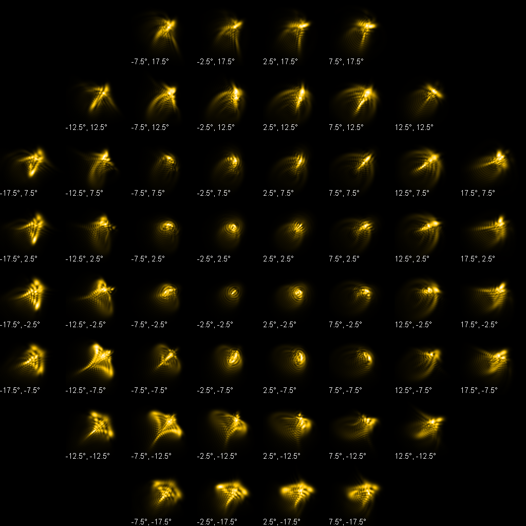
Fig. 9: Zemax PSFs across the focal plane. Credit: C. Paproth.
The following parameters are only applicable if Model = MappedFromFile:
MappedFromFile/Filename: Allowed values Path to Mapped PSF File
Path to the mapped PSFs in HDF5 format, holding precomputed Zemax PSFs. The most recent version of the precomputed PSFs can be downloaded from our FTP server.
MappedFromFile/NumberOfPixels: Allowed values \(> 0\) pixel
Number of pixels (in both directions) for which the PSF was generated.
MappedFromFile/ChargeDiffusionStrength: Allowed values \(> 0\) pixel
Charge diffusion has been modelled by a convolution with a Gaussian diffusion kernel, of which this is the standard deviation.
MappedFromFile/IncludeChargeDiffusion: Allowed values
yesandnoIndicates whether or not to include charge diffusion.
MappedFromFile/IncludeJitterSmoothing: Allowed values
yesandnoIndicates whether or not to include jitter smoothing. This is implemented as charge diffusion with a kernel width of 0.5 subpixels and alleviates the problem of jitter discontinuities. Only applicable in case
MappedFromFile/IncludeChargeDiffusion = False.
AnalyticNonGaussian:
The PSF is an analytical non-Gaussian model, the parameters of which are stored in a separate file. Fig. 10 shows the Analytic non-Gaussian model PSFs across the FPA.
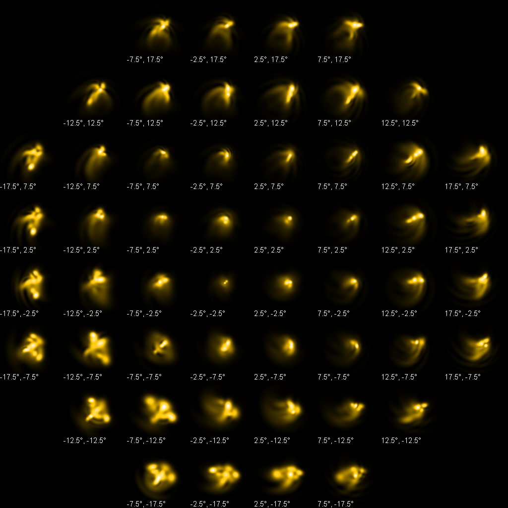
Fig. 10: Analytic non-Gaussian PSFs across the focal plane. Credit: C. Paproth.
The following parameters are only applicable if Model = AnalyticNonGaussian:
AnalyticNonGaussian/ParameterFileName: Path to Analytic PSF File
Path to the PSFs file in ascii format, holding the parameters characterising the analytical model. The most recent values for these parameters can be found in the file
inputfiles/apsf_N6000K_v2.txt. These model parameters have been derived from a best fit solution to the corresponding Zemax PSFs given by the fileinputfiles/PSF_Focus_0mu.hdf5.AnalyticNonGaussian/Sigma:
The width of the analytic non-Gaussian PSF, equal to sigma for a Gaussian PSF, can either be kept constant over the simulations or vary, according to the values in a file provided by the user.
AnalyticNonGaussian/Sigma/Source: Allowed values
ConstantValueandFromFileIndicates whether the value of the width of the analytic non-Gaussian PSF must be constant or is allowed to vary over time, according to the values in a user-provided file.
AnalyticNonGaussian/Sigma/ConstantValue: Allowed values \(> 0\) pixel
Width of the analytic non-Gaussian PSF, equal to sigma for a Gaussian PSF, in case it must remain the same over the duration of the whole simulation. This entry is only applicable if
Sigma/Source = ConstantValue.AnalyticNonGaussian/Sigma/FromFile: Allowed values Path to Analytic PSF Width file
If
AnalyticNonGaussian/Sigma/Source = FromFile, a time series for the width of the analytic non-Gaussian PSF must be provided in a ascii file. This file should contain columns, separated by a space, holding the following information:
- Time [s]
- Width of the PSF [pixels]
AnalyticGaussian:
Warning
Note that this very crude model was used for beta-testing and is thus not recommended!
The PSF is an elongated Gaussian (the symmetry axes being parallel to the \(x\) and \(y\) axis), for which the width and the height are given at the centre of the FOV and at \(18^{\circ}\) from the optical axis. The following parameters are only applicable if Model = AnalyticGaussian:
AnalyticGaussian/Sigma00: Allowed values \(> 0\) pixel
Standard deviation of the analytical Gaussian PSF in the \(x\) and \(y\) direction at the optical axis.
AnalyticGaussian/SigmaX18: Allowed values \(> 0\) pixel
Standard deviation of the analytical PSF in the \(x\) direction at 18 degrees from the optical axis.
AnalyticGaussian/SigmaY18: Allowed values \(> 0\) pixel
Standard deviation of the analytical PSF in the \(y\) direction at 18 degrees from the optical axis.
FEE
The FEE block of the configuration file contains all the information that is specific to the Front-End Electronics (FEE). The structure of this block is the following:
NominalOperatingTemperature: Allowed values \(> 0\) K
Nominal operating temperature of the FEE.
Temperature: Allowed values Nominal and FromFile
Indicates whether the temperature of the FEE should be fixed at the nominal operating temperature or temperature variations should be read from a file.
TemperatureFileName Allowed values Path to FEE Temperature File
If FEE/Temperature = FromFile, a temperature time series for the FEE must be provided in a ascii file. This file should contain two columns, separated by a space, holding the following information:
- Time [s]
- Operating temperature of the FEE [K]
ReadoutNoise: Allowed values \(\ge 0 \ \text{e}^- \, \text{pixel}^{-1}\)
Mean readout noise of the FEE. This is the same for both ADCs.
Gain:
The actual gain for the FEE will be different for both ADCs. A reference value is given for ADC1 and ADC2, and the difference should not exceed the specified allowed difference.
Gain/RefValueLeft: Allowed values \(> 0 \ \text{ADU} \, \mu\text{V}^{-1}\)
Reference value of the gain of ACD1 of the FEE at its nominal operating temperature.
Gain/RefValueRight: Allowed values \(> 0 \ \text{ADU} \, \mu\text{V}^{-1}\)
Reference value of the gain of ACD2 of the FEE at its nominal operating temperature.
Gain/Stability: Allowed values \(\ge 0 \ \text{ADU} \, \mu\text{V}^{-1} \, \text{K}^{-1}\)
Change in gain (for both ADCs) with temperature deviations from the nominal operating temperature
Gain/AllowedDifference: Allowed values \(\in [0, 100] \%\)
Percentage of the reference values for the gain of ADC1 and ADC2 that indicates the maximum allowed difference between these gain values.
ElectronicOffset:
The electronic offset or bias level is added to the digital signal in order to avoid negative readout values. The electronic offset can be measured in a prescan strip, which essentially consists of a few additional rows of the CCD. These rows only contain the electronic offset and the readout noise. This prescan strip consisting of NumPreScanRows rows will be stored in the output file. This is the same for both ADCs.
ElectronicOffset/RefValue: Allowed values \(\ge 0 \, \text{ADU} \, \text{pixel}^{-1}\)
Electronic offset or bias level at the nominal operating temperature of the FEE.
ElectronicOffset/Stability: Allowed values \(\ge 0 \, \text{ADU} \, \mu\text{V}^{-1} \, \text{K}^{-1}\)
Change in electronic offset (for both ADCs) with temperature deviations from the nominal operating temperature.
IncludeOverAndUnderShoot: Allowed values yes and no
Indicates whether or not to include F-FEE over-/undershoot.
Warning
Over-/undershoot is currently only availble for fast cameras (GroupID = Fast).
OverAndUnderShoot:
Over-/undershoot has been noticed in F-FEE measurements. Looking at the content of a readout register at any given time, the charges in any pixels will affect the next pixels in the readout register, further away from the readout register, e.g. at a distance \(\Delta x\). For a difference in signal between two such pixels, \(\Delta S\), the induced over-/undershoot will be:
\(a \cdot \Delta S \cdot \exp{(- \lambda \cdot \Delta x^b)}.\)
Both detector halves are treated independently.
OverAndUnderShoot/Strength: Allowed values \(> 0\)
Parameter \(a\) in the formula above.
OverAndUnderShoot/DecayRate: Allowed values \(> 0\)
Parameter \(\lambda\) in the formula above.
OverAndUnderShoot/DecaySpeed: Allowed values \(> 0\)
Parameter \(b\) in the formula above.
OverAndUnderShoot/Range: Allowed values \(> 0\) pixel
Maximum distance \(\Delta x\) over which a pixel in the readout register exerts over-/undershoot on other pixels in the readout register, further away from the readout electronics.
CCD
Position: Allowed values 1, 2, 3, 4, and Custom
The CCD position can be used to select a specific predefined CCD or a custom one. The predefined CCD positions are shown in the Fig. 11 and 12.
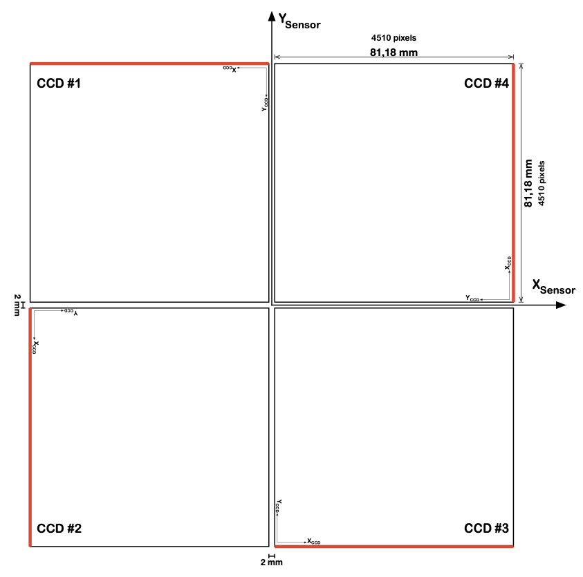
Fig. 11: Layout of the CCDs for the N-CAMs.
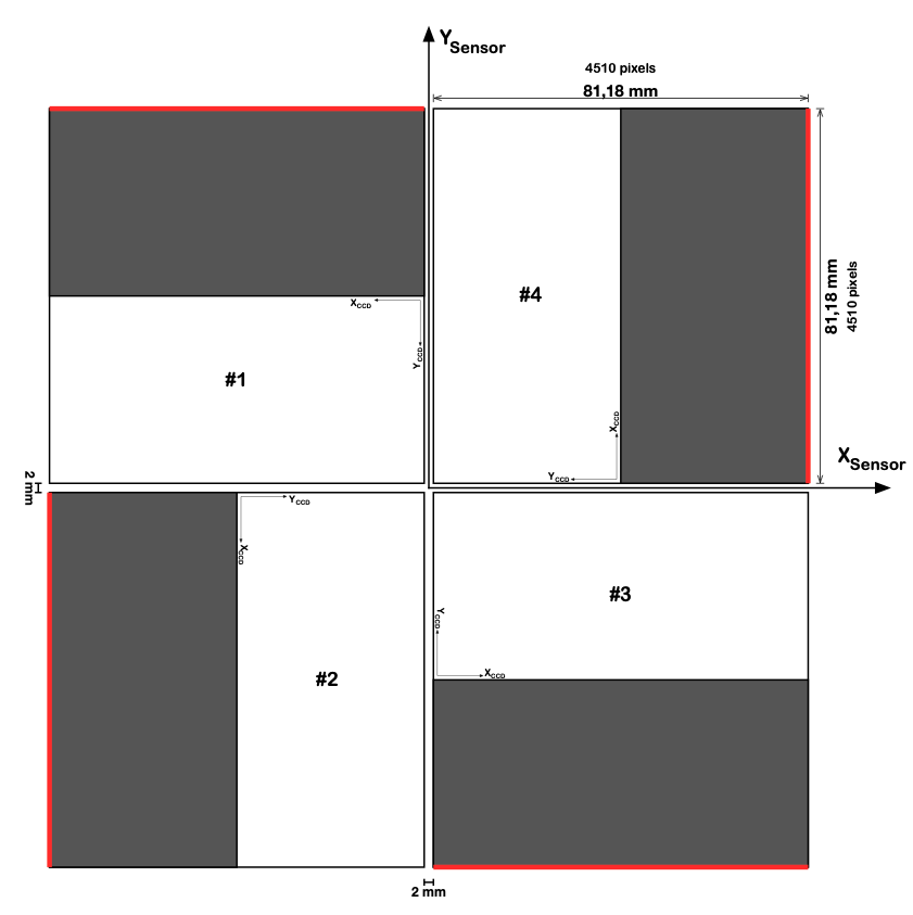
Fig. 12: Layout of the CCDs for the F-CAMs.
When you specify Position=Custom, the origin offset OriginOffsetX and OriginOffsetY, the orientation, number of rows, and columns, and the first exposed row of the CCD are read from the configuration parameters in the CCD block.
OriginOffsetX: Allowed values \(\in \mathbb{R}\) mm
Offset of the CCD origin from the centre of the optical plane (i.e. the intersection of the optical axis with the focal plane) in the y-direction. The origin of the CCD is defined as the point where the readout register is located. See Fig. 7 for more details (\(\Delta x_{\rm CCD}\)). Parameter used if Position = Custom.
OriginOffsetY: Allowed values \(\in \mathbb{R}\) mm
Offset of the CCD origin from the centre of the optical plane (i.e. the intersection of the optical axis with the focal plane) in the y-direction. The origin of the CCD is defined as the point where the readout register is located. See Fig. 7 for more details (\(\Delta y_{\rm CCD}\)). Parameter used if Position = Custom.
Orientation: Allowed values \(\in [0, 360]\) deg
Orientation angle of the CCD w.r.t. the orientation of the focal plane, measured counterclockwise and expressed in degrees. This rotation is performed around the offset origin of the CCD. See Fig. 7 for more details (\(\gamma_{\rm CCD}\)). Parameter used if Position = Custom
NumColumns: Allowed values \(\ge 0\) pixel
Number of pixels of the CCD in the x-direction (i.e. number of columns). Parameter used if Position = Custom.
NumRows: Allowed values \(\ge 0\) pixel
Number of pixels of the CCD in the y-direction (i.e. number of rows). Parameter used if Position = Custom.
FirstRowExposed: Allowed values \(\ge 0\) pixel
Row index of the first row in the CCD that is illuminated (the row closest to the readout register is row 0). Parameter used if Position = Custom.
TimeShift: Allowed values \(\ge 0\) s
Time shift between the readout of the CCDs [s]. Parameter used if Position = Custom.
PixelSize: Allowed values \(\ge 0\) micron
Nominal pixel size.
BFE:
Brighter-Fatter Effect (BFE) modelled following the method proposed by Guyonnet et al. 2015.
BFE/CoefficientsFileName: Path to BFE Coefficients file
Path to the HDF5 file comprising the coefficients
afor the BFE.
Gain:
The actual gain for the CCD will be different for both detector halves. A reference value is given for both halves, and the difference should not exceed the specified allowed difference AllowedDifference given below.
Gain/RefValueLeft: Allowed values \(> 0 \ \mu\text{V}/\text{e}^-\).
Reference value of the gain of the left- and right-hand side of the CCD at its nominal operating temperature.
Gain/RefValueRight: Allowed values \(> 0 \ \mu\text{V}/\text{e}^-\).
Reference value of the gain of ACD2 of the FEE at its nominal operating temperature.
Gain/Stability: Allowed values \(\in \mathbb{R} \ \mu\text{V}/\text{e}^-/\text{K}\)
Change in gain (for both CCD halves) with temperature deviations from the nominal operating temperature.
Gain/AllowedDifference: Allowed values \(\in [0, 100] \ \mu\text{V}/\text{e}^-\).
Percentage of the reference values for the gain of the left- and right-hand side of the CCD that indicates the maximum allowed difference between these gain values.
Gain/Nonlinearity: Allowed values \(\in \{\mathbb{R}, \mathbb{R}, \mathbb{R}\}\)
CCD gain non-linearity model coefficients of the polynomial:
\(O = B + I + a0 + a_1 \cdot I + a_2 \cdot I^2\),
with \(O\) being the output signal [ADU], \(B\) the bias level [ADU], and \(I\) is the input signal [ADU].
QuantumEfficiency:
Quantum efficiency is the ratio of the number of collected electrons to the number of incident photons, considering the passband and the spectral energy distribution of the stars given the Fluxm0 and the magnitude of the stars in the star catalogue.
QuantumEfficiency/MeanQuantumEfficiency: Allowed values \(\in [0, 1]\)
Mean throughput efficiency due to quantum efficiency (i.e. the mean over all pixels of one detector).
QuantumEfficiency/MeanAngleDependency: Allowed values \(\in [1, 2]\)
Reference angle for the throughput efficiency due to the quantum efficiency.
FullWellSaturation: Allowed values \(> 0 \ \text{e}^- \, \text{pixel}^{-1}\)
Full-well saturation limit of a single CCD pixel. If a pixels receives more electrons than its full-well saturation limit, the additional electrons flow evenly distributed in positive and negative charge-transfer direction, a phenomenon called blooming. The electrons reaching the edge of the CCD will not be detected.
DigitalSaturation: Allowed values \(> 0 \ \text{ADU} \ ,\text{pixel}^{-1}\)
Digital saturation limit of the CCD to which pixel values are topped off. This value depends on the A/D convertor of the detector. For a 16-bit convertor, the digital saturation limit is \(655\,36\) ADU. The gain of the front-end electronics and detector should be such that the full-well saturation results in values below the digital saturation limit.
ReadoutNoise: Allowed values \(\ge 0 \ \text{e}^- \, \text{pixel}^{-1}\)
Mean readout noise of the detector. Readout noise occurs due to the imperfect nature of the CCD amplifiers. When the electrons are transferred to the amplifier, the induced voltage is measured. However, this measurement is not perfect, but gives a value which is on average too high by an amount of the readout noise, with the square-root of the readout noise as standard deviation (we add the readout noise of the FEE and the CCD in quadrature).
SerialTransferTime: Allowed values \(> 0\) ns
Time required to shift the content of the readout register over one pixel, towards the output node. This is not only relevant for the image area but also for the serial prescan (i.e. bias register map) and the serial over-scan (which has not been implemented).
ParallelTransferTime: Allowed values \(> 0 \, \mu\text{s}\)
Time required to shift the charges one row down (towards the readout register) in case the readout register will be read out by the FEE. The difference with ParallelTransferTimeFast is due to two delay parameters recommended by Teledyne e2v for clock settling. Settling times are to ensure one clock has reached its low level before another clock starts to rise. It ensures good charge transfer, as without it you could cause charge to be lost. This is particularly the case when dealing with the (parallel) transfer into the readout register, as the rise and fall times of the image clocks are a lot slower than those of the register clocks.
ParallelTransferTimeFast: Allowed values \(\ge 0 \, \mu\text{s}\)
Time required to shift the charges one row down (towards the readout register) in case the readout register will not be read out by the FEE. In that case clock settling is not needed, hence the difference with ParallelTransferTime.
ReadoutMode:
This determines how the CCD is read out. The readout mode can either be Nominal or Partial. Nominal readout mode mode will read out all the 4510 rows starting at row 0 for normal cameras, and only 2255 rows starting at row 2255 for the fast cameras (the lower half of the CCD is shielded off). For the Partial readout mode, only certain rows are read out. These rows can be on the upper half of the CCD for the fast cameras and on the entire CCD for the normal cameras.
ReadoutMode/ReadoutMode: Allowed values
NominalandPartialReadoutMode/Partial:
Configuration settings for when
ReadoutMode = Partial:ReadoutMode/Partial/FirstRowReadout: Allowed values \(\ge 0\) pixel
First row that will be read out by the FEE.
ReadoutMode/Partial/NumRowsReadout: Allowed values \(\ge 0\) pixel
Numbers of rows that will be read out by the FEE.
FlatfieldNoiseRMS: Allowed values \(\ge 0\)
Local Pixel Response Non-Uniformity (PRNU), defined as the standard deviation in the signal level (\(S_i\)), divided by the mean signal (\(\overline{S}\)):
\(\text{PRNU} = \frac{\sqrt{\frac{1}{N} \sum_{i=1}^{N} (S_i - \overline{S})^2}}{\overline{S}}\)
RelativeTransmissivity:
On top of the (time-dependent) transmission efficiency, the overall relative transmissivity should be taken into account. This decrease in efficiency with distance to the optical axis, comprises the following contributions:
Natural vignetting (brightness attenuation towards the edges of the FOV, introduced by the view factor of the entrance pupil)
Mechanical vignetting (due to the undersized mask at the entrance pupil), incl. total blockage of all incoming radiation beyond the edge of the FOV
Glass absorption + anti-reflective coating
RelativeTransmissivity/Coefficients: Allowed values \(> \{0, 0, 0\}\)
Coefficients \(k_1, \, k_2, \, k_3\) for the polynomial that converts the distance from the optical axis, \(\theta\) (expressed in degrees), to the variation in the overall relative transmissivity (expressed in percentage):
\(P(\theta) = k_1 \cdot \theta^2 + k_2 \cdot \theta^4 + k_3 \cdot \theta^6\).
RelativeTransmissivity/RadiusFOV: Allowed values \(> 0\) deg
Radius of the FOV. Beyond this radius all incoming flux (apart from the cosmic hits) is shielded off.
RelativeTransmissivity/ExpectedValue: Allowed values \(\in [0, 1]\)
Expected value of the throughput efficiency due to the overall relative transmissivity (i.e. the mean over all pixels of one detector, within the FOV).
Polarization:
Optical elements induce a preferred direction for the propagation of light. This effect is called polarisation.
Polarization/ExpectedValue: Allowed values \(\in [0, 1]\)
Expected value of the throughput efficiency due to polarisation (i.e. the mean over all pixels of one detector). Currently no information on the angle dependency of polarisation is available and hence this value will be used for the whole FOV, until further notice.
Contamination:
The contribution to contamination is two-fold:
Particulate contamination is the unintended presence of particles on (optical) surfaces, which leads to straylight and influences the effciency
Molecular contamination is caused chiefly by outgassing of materials in the first phase of the mission and affects all surfaces (the down side of L2 and the CCD will be affected the most).
Contamination/ParticulateContaminationEfficiency: Allowed values \(\in [0, 1]\)
Throughput efficiency due to particulate contamination.
Contamination/MolecularContaminationEfficiency: Allowed values \(\in [0, 1]\)
Throughput efficiency due to molecular contamination.
DarkSignal:
Dark signal is the relatively small electric current that is generated in the CCD when no outside radiation is entering the device.
DarkSignal/DarkCurrent: Allowed values \(> 0 \ \text{e}^-\)
Dark current of detector. This is the nominal value of the dark signal.
DarkSignal/DSNU: Allowed values \(\in [0, 100] \%\)
Dark Signal Non-Uniformity (DSNU), expressed as a percentage of the dark current. This is the systematic (fixed-pattern) deviation of a pixel’s dark current from its nominal value.
DarkSignal/Stability: Allowed values \(\ge 0 \ \text{K}^{-1} \, \text{s}^{-1}\)
Temperature stability of the dark current.
CTI:
Because of detector defects, electrons can get trapped in the readout process. The trapped charge ends up getting dissociated from its original pixel and eventually gets released into another pixel. The result is that the original image gets smeared out in the direction away from the readout amplifier (visible in the appearance of charge trails). This is known as Charge-Transfer Inefficiency (CTI).
The charge trails impact photometry, noise, and astrometry of sources. CTI removes flux from the central pixel and thus degrades the expected S/N for an observation. CTI trails bias measurements of source along the trail direction, which can severely impact high-precision astrometry.
CTI/Model: Allowed values
Simple,Short2013,Short2013FromFilePlatoSim offers two implementation of the CTI:
The simple implementation (
Simple) assumes that for each row transfer (in the direction of the readout register) a fraction of the charge is not transferred to the next row, but stays behind. It will be released by later row transfers.A more sophisticated implementation (
Short2013) is based on the paper by Short et al. (2013), in which only parallel readout is taken into account.CTI/Simple:
The simple implementation (
Simple) assumes that for each row transfer (in the direction of the readout register) a fraction of the charge is not transferred to the next row, but stays behind. It will be released by later row transfers.CTI/Simple/MeanCTE: Allowed values \(\in [0, 1]\)
Mean CTE of the detector. The fraction of the charge that is successfully transferred from one row to the next row is expressed by this parameter.
CTI/Short2013:
This is the more realistic modelling four hole-pair species:
CTI/Short2013/Beta: Allowed values \(> 0\)
Exponent \(\beta\) in Eq. (1) of Short et al. (2013) describing the relationship between the volume of the charge cloud (\(V_c\)), the number of electrons in a pixel (\(N_e\)), the full-well capacity in electrons (FWC), and the assumed maximum geometrical volume that electrons can occupy within a pixel (\(V_g\)):
\(\frac{V_c}{V_g} = \left(\frac{N_e}{FWC}\right)^{\beta}\).
CTI/Short2013/Temperature: Allowed values \(\ge 0\) K
Temperature \(T\) that is used to calculated the thermal velocity \(v_t\) of the electrons:
\(v_t = \frac{3 k T}{m_e^*}\),
where \(k\) is the Boltzmann constant and \(m_e^*\) is the effective electron mass in silicon, which we approximate by half the free electron rest mass.
CTI/Short2013/NumTrapSpecies: Allowed values \(> 0\)
Number of trap species that is used in the CTI model by Short et al. 2013.
CTI/Short2013/TrapDensity:
We assume the trap density for each of the considered trap densities to increase linearly over time (in absence of charge injection).
CTI/Short2013/TrapDensity/BOL: Allowed values \(> \{0, 0, 0, 0\} \, \text{traps} \, \text{pixel}^{-1}\)
Array holding the trap density \(n_t\) at BOL for each of the considered trap species. This is used to calculate the \(\gamma\) value in Eq. (22) of Short et al. (2013).
CTI/Short2013/TrapDensity/EOL: Allowed values \(> \{0, 0, 0, 0\} \, \text{traps} \, \text{pixel}^{-1}\)
Array holding the trap density \(n_t\) at EOL for each of the considered trap species. This is used to calculate the \(\gamma\) value in Eq. (22) of Short et al. (2013).
CTI/Short2013/TrapCaptureCrossSection: Allowed values \(> \{0, 0, 0, 0\} \, \text{m}^2\)
Array holding the trap capture cross-section \(\sigma\) for each of the considered trap species. This is used to calculated the \(\alpha\) value in Eq. (22) of Short et al. (2013). In this formula, the charge transfer time is used as value for \(t\).
CTI/Short2013/ReleaseTime: Allowed values \(> \{0, 0, 0, 0\}\) s
Array holding the trap release time constants \(\tau_r\) for each of the considered trap species.
CTI/Short2013FromFile:
Allows to specify trap densities that vary spatially over the CCD.
CTI/Short2013FromFile/CTIFileName: Allowed values Path to CTI File
Path to the CTI file holding information about trap densities.
ChargeInjection:
Settings for the charge injection.
ChargeInjection/InjectionLevel: Allowed values \(\in [0, 100] \, \%\)
Percentage of the full well to be filled.
ChargeInjection/RowInterval: Allowed values \(\in [1, n-n_{\text{CCD}}]\) pixel
The interval around which Charge Injection will happen. For a value of \(n\), the charge will be injected every \(n\)-th row of the CCD after the
FirstRow:ChargeInjection/FirstRow: Allowed values \(> 0\) pixel
The first row that will be injected with charge.
NominalOperatingTemperature: Allowed values \(> 0\) K
Nominal operating temperature of the CCD.
Temperature: Allowed values Nominal and FromFile
Indicates whether the temperature of the CCD should be fixed at the nominal operating temperature or temperature variations should be read from a file.
TemperatureFileName: Allowed values Path to file ( CCD Temperature File)
Path to the file with the temperature variations of the CCD (absolute path or relative to project home).
IncludeFlatfield: Allowed values yes and no
Indicates whether or not to include the flatfield.
IncludeDarkSignal: Allowed values yes and no
Indicates whether or not to include dark signal.
IncludeBFE: Allowed values yes and no
Indicates whether or not to inlcude the Brighter Fatter Effect
IncludePhotonNoise: Allowed values yes and no
Indicates whether or not to include photon noise.
IncludeReadoutNoise: Allowed values yes and no
Indicates whether or not to include readout noise.
IncludeCTIeffects: Allowed values yes and no
Indicates whether or not to include CTI effects.
IncludeChargeInjection: Allowed values yes and no
Indicates whether or not to include charge injection
IncludeOpenShutterSmearing: Allowed values yes and no
Indicates whether or not to include open-shutter smearing effects.
IncludeQuantumEfficiency: Allowed values yes and no
Indicates whether or not to include loss of throughput efficiency due to quantum efficiency.
IncludeRelativeTransmissivity: Allowed values yes and no
Indicates whether or not to include the overall relative transmissivity.
IncludePolarization: Allowed values yes and no
Indicates whether or not to include loss of throughput efficiency due to polarisation.
IncludeParticulateContamination: Allowed values yes and no
Indicates whether or not to include loss of throughput efficiency due to particulate contamination.
IncludeMolecularContamination: Allowed values yes and no
Indicates whether or not to include loss of throughput efficiency due to molecular contamination.
IncludeConvolution: Allowed values yes and no
Indicates whether or not the subpixel map must be convolved with the PSF. This applies only to the Gaussian and the mapped PSF. The analytic non-Gaussian PSF is generated directly in pixel space.
IncludeFullWellSaturation: Allowed values yes and no
Indicates whether or not to apply full-well saturation.
IncludeDigitalSaturation: Allowed values yes and no
Indicates whether or not to apply digital saturation.
IncludeQuantisation: Allowed values yes and no
Indicates whether or not to apply quantisation. This includes:
- Applying gain (FEE and CCD), hence converting from electrons to ADUs
- Adding electronic offset
- Forcing the ADU values to be integers
- Applying digital saturation (can be switched off separately using
IinclDigitalSaturation).
Subfield
The SubField block of the configuration file contains all the information about the subfield of the CCD that is modelled by the simulation. The structure of this block is the following:
Figure 11 shows a schematic representation of the subfield and the parameters required to define it. The CCD focal plane array shows also the metallic shields of the F-CAM (purple colored areas).
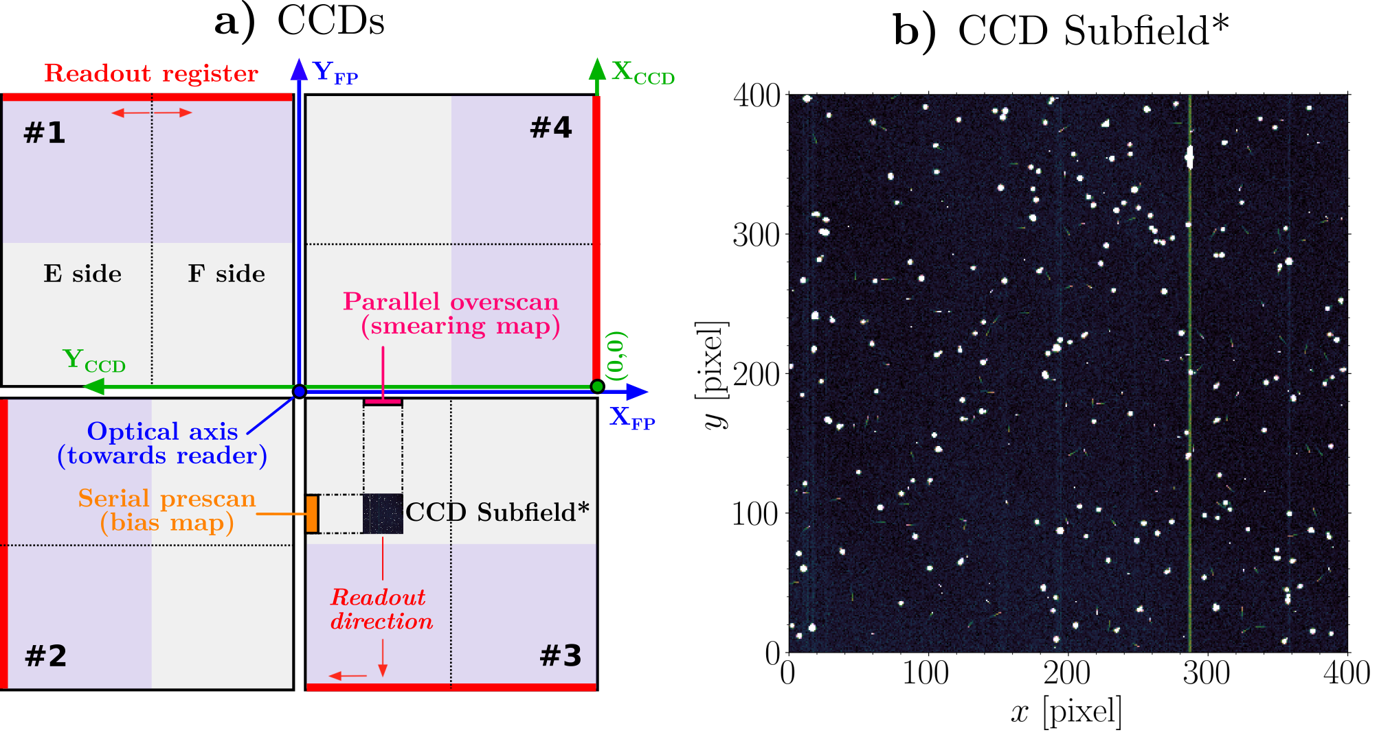
Fig. 11: Left: CCD focal plane with location subfield. Right: Simulated CCD subfield.
ZeroPointRow: Allowed values \(> 0\) pixel
Row of the origin of the subfield in the detector.
ZeroPointColumn: Allowed values \(> 0\) pixel
Column of the origin of the subfield in the detector.
NumColumns: Allowed values \(\ge 6\) pixel
Number of columns in the subfield.
NumColumns: Allowed values \(\ge 6\) pixel
Number of rows in the subfield.
NumBiasPrescanRows: Allowed values \(\ge 0\) pixel
Number of rows in the prescan strip (see Fig. 11). There are two such strips, on either side of the detector image (serial prescan and overscan), and they contain the electronic offset and readout noise of the adjacent detector half.
This parameter is configurable (and not fixed to the number of rows in the detector or the subfield), because we want: 1) to avoid the bias maps to take up too much space in the output file, and 2) be able to do accurate bias correction for the photometric reduction (thus want to avoid small noisy bias maps).
NumBiasPrescanColumns: Allowed values \(\ge 0\) pixel
Number of columns in the prescan strip (see Fig. 11). There are two such strips, on either side of the detector image (serial prescan and overscan), and they contain the electronic offset and readout noise of the adjacent detector half.
NumSmearingOverscanRows: Allowed values \(\ge 0\) pixel
Number of rows in the parallel overscan strip (see Fig. 11). This strip is located at the top of the sub-field that is modelled in detail and contains the star smearing due to the absence of a shutter. The flux in this strip is also affected by the electronic offset, readout noise, and shot noise. Not included are the PRNU, cosmic hits, and charge-transfer inefficiency (CTI).
SubPixels: Allowed values \(\in [1, 128]\) subpixel
Number of subpixels squared. If you want a pixel of \(16 \times 16 = 256\) subpixels, you should set this value to 16 subpixels. By default this parameter is only 8 subpixels to keep the computational resources low.
Photometry
The Photometry block of the configuration file contains all information to run photometry. The structure of this block is the following:
PlatoSim utilises the optimal aperture photometry algortihm from Marchiori et al. (2019). This method is optimised to lower the photometric noise relevant for planet transit searches. This algorithm allows to update the aperture mask with a user defined interval. Fig. 12 shows an example of an extracted light curve for a \(V=11\) star using a mask-update of 14 days (enhanced by the 1 hour running median filter shown in green).
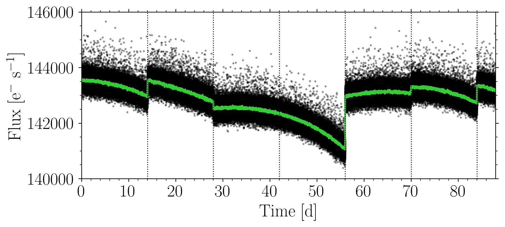
Fig. 12: Optimal aperture photometry with mask-updates every 14 days.
IncludePhotometry: Allowed values yes and no
Indicates whether or not photometry should be run.
ContaminationRadius: Allowed values \(> 0\) pixel
Radius around a target within which sources are considered contaminants when calculating the photometry for that target.
MaskUpdateInterval: Allowed values \(> 0\) days
Update interval to update the photometry mask.
TargetFileName: Allowed values Path to Photometry List file
Path of the file comprising the list of targets identifiers (as listed in the star catalogue in a single column). The path to the photometry list can be an absolute path or relative to the project location.
Random seeds
The RandomSeeds block of the configuration file contains all the seeds for random-number generation in the simulator. The structure of this block is the following:
Below each random seed can be set to a value of -1, which imply that the computer time at the start of the simulation will be used. That way, the fast-forward of the random generator when using Slurm is no longer needed (which is better for performance reasons). Note that the actual value that is used, will be written to the output HDF5 file.
ReadOutNoiseSeed: Allowed values \(> 0 \, \text{and} \, -1\)
Seed for the random-number generator used for the readout noise.
PhotonNoiseSeed: Allowed values \(> 0 \, \text{and} \, -1\)
Seed for the random-number generator used for the photon noise.
JitterSeed: Allowed values \(> 0 \, \text{and} \, -1\)
Seed for the random-number generator used for the jitter.
FlatFieldSeed: Allowed values \(> 0 \, \text{and} \, -1\)
Seed for the random-number generator used for the flatfield.
DriftSeed: Allowed values \(> 0 \, \text{and} \, -1\)
Seed for the random number generator used for the drift.
CosmicSeed: Allowed values \(> 0 \, \text{and} \, -1\)
Seed for the random-number generators for the cosmics.
DarkSignalSeed: Allowed values \(> 0 \, \text{and} \, -1\)
Seed for the random-number generators for the dark signal.
Warning
To avoid jumps in the power spectrum when using auto-generated red noise jitter and/or drift models, it is advised to take special care in setting the random seeds. Another options is to generate these red noise time series for the whole simulation beforehand, write these values to a file, and reading in that file when simulating the different chunks.
Control HDF5 content
The ControlHDF5Content block of the configuration file contains all the seeds for random-number generation in the simulator. The structure of this block is the following:
GroupByExposure: Allowed values yes and no
This entry controls the exact output structure of the groups StarPositions, PointLikeGhostPositions, ExtendedGhostPositions, and Cosmics:
- If
yes: all information is saved in folders per exposure - if
no: all information is saved per star ID.
For long baseline simulations (more than \(100\,000\) exposures), we recommend to use the latter option since this can significantly lower the computational resources (time and memory). Note that the information about the cosmic rays are never saved per star, however, it is saved into subfolders of 1000 exposures each if GroupByExposure = no.
WritePixelImages: Allowed values yes and no
Indicates whether or not the pixel maps must be stored in the output file.
WriteBiasMaps: Allowed values yes and no
Indicates whether or not the bias register maps must be stored in the output file.
WriteSmearingMaps: Allowed values yes and no
Indicates whether or not the smearing maps must be stored in the output file.
WriteFlatfieldMap: Allowed values yes and no
Indicates whether or not the flatfield maps must be stored in the output file.
WriteThroughputMaps: Allowed values yes and no
Indicates whether or not the throughput maps must be stored in the output file.
WriteTransmissionEfficiency: Allowed values yes and no
Indicates whether the Transmission Efficiency should be stored in the output file.
WriteBackgroundMaps: Allowed values yes and no
Indicates whether the Sky Background maps hould be stored in the output file. If a constant background values is used this will be a single float value and not an image map.
WriteCTI: Allowed values yes and no
Indicates whether the CTI maps hould be stored in the output file. This is the trap density maps at BOL and EOL for each species.
WriteSubPixelImages: Allowed values yes and no
Indicates whether or not the sub-pixel maps must be stored in the output file. Only do this for a small number of exposures, as this takes up a lot of space. Note that this only takes into account the effects that are applied until right before the re-binning (see PlatoSim’s control flow).
WriteHighResolutionPSF: Allowed values yes and no
Indicates whether or not a high resolution image of the PSF should be stored in the output file. This feature does not work for Analytic Gaussian PSF.
WriteDiffusedPSF: Allowed values yes and no
Indicates whether or not a high resolution image of the PSF with diffusion applied to it should be stored in the output file. This features only works for the mapped PSF and takes a long time to compute.
WriteACS: Allowed values yes and no
Indicates whether or not the camera Yaw, Pitch and Roll should be stored in the output file. This scales with the number of exposures.
WriteTelescopeACS: Allowed values yes and no
Indicates whether or not the platform Yaw, Pitch and Roll should be stored in the output file. This scales with the number of exposures.
WriteStarCatalog: Allowed values yes and no
Indicates whether or not the starcatalog should be stored in the output file.
WriteStarPositions: Allowed values yes and no
Indicates whether or not the star positions should be stored in pixel and focal plane coordinates in the output file. This scales with the number of exposures and the number of stars in the sub-field.
WriteGhostPositions: Allowed values yes and no
Indicates whether or not the ghost positions should be stored in pixel and focal plane coordinates in the output file. This scales with the number of exposures and the number of stars in the sub-field.
WriteCosmics: Allowed values yes and no
Indicates whether or not the columns, rows and flux of the cosmics should stored in the output file. This scales with the number of exposures.
Control TCP connection
The ControlTcpConnection block in the configuration file is read from a network. The structure of this block is the following:
SendImagettesToClients: Allowed values yes and no
Indicates whether or not the simulated imagettes should be sent to the client.
GetWindowPositionsFromServer: Allowed values yes and no
Indicates whether or not the window positions should be taken from a server and be updated in upcoming simulations.
WindowPositionServerAddress: Allowed values String with TPC address
Address from which to read the window positions in case this is requested (GetWindowPositionsFromServer = yes).
JitterServerAddress: Allowed values String with TPC address
Address from which to read the jitter positions.
ImagetteClientAddress: Allowed values String with TPC address
Client address to which to send the simulated imagettes in case this is requested (SendImagettesToClients = yes).
WindowPositionSocketTimeout: Allowed values \(> 0\)
Number of seconds of not receiving window positions (from the window position server), after which the connection to that server is regarded as stalled / broken.
JitterSocketTimeout: Allowed values \(> 0\)
Number of seconds of not receiving jitter positions (from the jitter server), after which the connection to that server is regarded as stalled / broken.
Camera Groups
Warning
You are not supposed to alter this section of the configuration file!
The CameraGroups block in the configuration file is used in case of a predefined camera groups (1, 2, 3, 4, or Fast) was selected via the Telescope/GroupID parameter. The structure of this block is the following:
For more information, consult our technical note: PLATO-KUL-PL-TN-0001.
CCD Positions
Warning
You are not supposed to alter this section of the configuration file!
The CCDPositions block in the configuration file is used in case of a predefined CCD position (1, 2, 3, or 4) was selected via the CCD/Position parameter. The structure of this block is the following:
For more information, consult our technical note: PLATO-KUL-PL-TN-0001.
Supplementary files
Depending on you configuration, some additional files may be required. We here provide a table to quickly query the one(s) that may be of your interest:
Overview of Supplementary Files
- Star Catalog File: a star catalog file of the region of the sky of interest
- Variable Source List: a star variable list of the sources in the star catalog
- Jitter File: a time series for the jitter angles
- Drift File: a time series for the drift angles
- Focal Plane Orientation File: a time series for the focal-plane orientation
- Focal Length File: a time series for the focal length
- Orbit File: a time series of the spacecraft position and velocity
- Field Distortion: two time series for the field distortion coefficients and their inverse
- Mapped PSF File: a file with precomputed Zemax PSFs
- Analytic PSF File: a file with parameters of the analytic non-Gaussian PSF
- Analytic PSF Width: a time series for the width of the analytic non-Gaussian PSF
- FEE Temperature File: a time series for the operating temperature of the FEE
- BFE Coefficients: a file with the coefficients of the BFE model
- CTI File: a file with trap dencities that may vary spatially across the CCD
- CCD Temperature File: a time series for the operating temperature of the CCD
- Photometry List: a photometry list of the sources from the star catalog
A few notes about the provided time series:
- The path to each file above can be given as an absolute path or relative to the project location.
- Always secure that the duration of your time series is greater than the planned simulation.
- PlatoSim will automatically interpolate the provided time series if time step is larger that the cadence.
PSF data packages
If you want to use realistic PSF models instead of a Gaussian, you can download these from out FTP server. The default file for most users (in focus PSF at a 6000K stellar effective temperature) can be found here.
Default PSF (at 6000K):
Out off focus PSF (at 6000K):
- Distortion: +100 mu
- Distortion: +80 mu
- Distortion: +60 mu
- Distortion: +40 mu
- Distortion: +20 mu
- Distortion: +10 mu
- Distortion: -10 mu
- Distortion: -20 mu
- Distortion: -40 mu
- Distortion: -60 mu
- Distortion: -80 mu
- Distortion: -100 mu
PSF at different stellar effective temperatures: